Examples

It is recommended that you go through the quick start guide before reading this page.

This page is generated by a Jupyter notebook which can be opened and run in Binder or Google Colab by clicking on the above badges. To run it in Google Colab, first you need to install PyMinimax and a newer version of scikit-learn in Colab:

!pip install pyminimax scikit-learn==0.23

Random Points in 2D

In this example we perform minimax linkage clustering on a toy dataset of 20 random points in 2D:

import numpy as np
from pandas import DataFrame

np.random.seed(0)
X = np.random.rand(20, 2)

DataFrame(X, columns=['x', 'y'])

	x	y
0	0.548814	0.715189
1	0.602763	0.544883
2	0.423655	0.645894
3	0.437587	0.891773
4	0.963663	0.383442
5	0.791725	0.528895
6	0.568045	0.925597
7	0.071036	0.087129
8	0.020218	0.832620
9	0.778157	0.870012
10	0.978618	0.799159
11	0.461479	0.780529
12	0.118274	0.639921
13	0.143353	0.944669
14	0.521848	0.414662
15	0.264556	0.774234
16	0.456150	0.568434
17	0.018790	0.617635
18	0.612096	0.616934
19	0.943748	0.681820

Below is the dendrogram.

import matplotlib.pyplot as plt
from pyminimax import minimax
from scipy.spatial.distance import pdist
from scipy.cluster.hierarchy import dendrogram

Z = minimax(pdist(X), return_prototype=True)

plt.figure(figsize=(10, 4))
dendrogram(Z[:, :4])
plt.show()

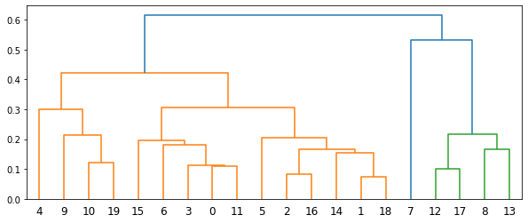
A unique advantage of minimax linkage hierarchical clustering is that every cluster has a prototype selected from the original data. This is a representative data point of the cluster.

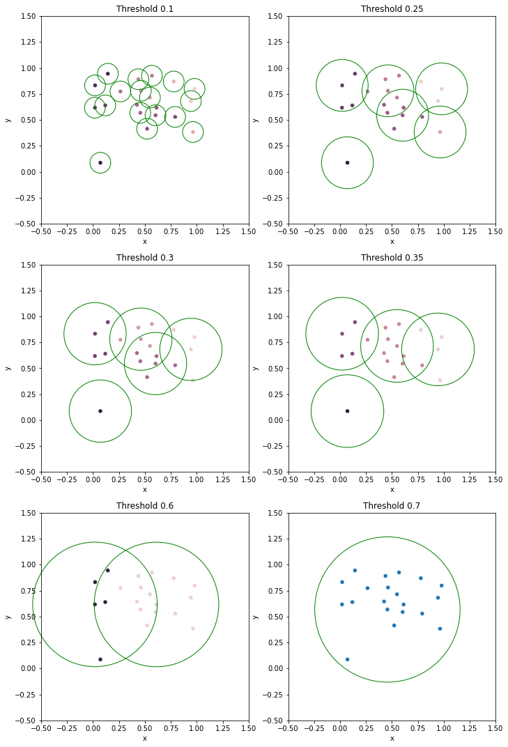
The threshold used to cut the dendrogram is also interpretable. Suppose the dendrogram is cut at threshold \(t\), splitting the data into clusters \(G_1, G_2, \ldots\) with corresponding prototypes \(p_1, p_2, \ldots\). Then, for any \(i\), all data points in \(G_i\) must be in the circle centered at \(p_i\) with radius \(t\). That is, the distance from the prototype of a cluster to any data point in the same cluster must be less than or equal to \(t\).

Here we draw the clusters and the circles for various thresholds. The data points at the center of the circles are the prototypes.

import seaborn as sns
from pandas import DataFrame
from pyminimax import fcluster_prototype

cuts = [0.1, 0.25, 0.3, 0.35, 0.6, 0.7]

fig, axs = plt.subplots(3, 2, figsize=(10, 15))

for ax, cut in zip(axs.ravel(), cuts):
    clust_proto = fcluster_prototype(Z, t=cut, criterion='distance')

    df = DataFrame(np.concatenate([X, clust_proto], axis=1), columns=['x', 'y', 'clust', 'proto'])
    sns.scatterplot(data=df, x='x', y='y', hue='clust', legend=None, ax=ax)

    ax.set(xlim=(-0.5, 1.5), ylim=(-0.5, 1.5), aspect=1, title=f'Threshold {cut}')
    protos = np.unique(df['proto'].map(int).values)
    for proto in protos:
        circle = plt.Circle(X[proto], cut, edgecolor='g', facecolor='none', clip_on=False)
        ax.add_patch(circle)

fig.tight_layout()
plt.show()

Hand-Written Digits

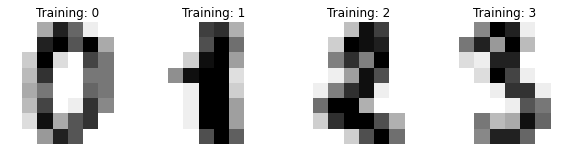
In this example we perform minimax linkage clustering on images of hand-written digits 1, 4 and 7. The data we use is a subset of the scikit-learn hand-written digit images data. The below code from its documentation prints the first few images in this dataset.

import matplotlib.pyplot as plt
from sklearn import datasets

digits = datasets.load_digits()

_, axes = plt.subplots(nrows=1, ncols=4, figsize=(10, 3))
for ax, image, label in zip(axes, digits.images, digits.target):
    ax.set_axis_off()
    ax.imshow(image, cmap=plt.cm.gray_r, interpolation='nearest')
    ax.set_title('Training: %i' % label)

First we load the data in a pandas DataFrame, and filter out images that are not 1, 4 or 7. The resulting DataFrame digits147 has 542 rows, each having 65 values. The first 64 are a flattened \(8\times 8\) matrix representing the image, and the last value in the target column indicates this image is a 1, 4 or 7.

digits = datasets.load_digits(as_frame=True)['frame']
digits147 = digits[digits['target'].isin([1, 4, 7])].reset_index(drop=True)
digits147

	pixel_0_0	pixel_0_1	pixel_0_2	pixel_0_3	pixel_0_4	pixel_0_5	pixel_0_6	pixel_0_7	pixel_1_0	pixel_1_1	...	pixel_6_7	pixel_7_0	pixel_7_1	pixel_7_2	pixel_7_3	pixel_7_4	pixel_7_5	pixel_7_6	pixel_7_7	target
0	0.0	0.0	0.0	12.0	13.0	5.0	0.0	0.0	0.0	0.0	...	0.0	0.0	0.0	0.0	11.0	16.0	10.0	0.0	0.0	1
1	0.0	0.0	0.0	1.0	11.0	0.0	0.0	0.0	0.0	0.0	...	0.0	0.0	0.0	0.0	2.0	16.0	4.0	0.0	0.0	4
2	0.0	0.0	7.0	8.0	13.0	16.0	15.0	1.0	0.0	0.0	...	0.0	0.0	0.0	13.0	5.0	0.0	0.0	0.0	0.0	7
3	0.0	0.0	0.0	0.0	14.0	13.0	1.0	0.0	0.0	0.0	...	0.0	0.0	0.0	0.0	1.0	13.0	16.0	1.0	0.0	1
4	0.0	0.0	0.0	8.0	15.0	1.0	0.0	0.0	0.0	0.0	...	0.0	0.0	0.0	0.0	10.0	15.0	4.0	0.0	0.0	4
...	...	...	...	...	...	...	...	...	...	...	...	...	...	...	...	...	...	...	...	...	...
537	0.0	0.0	0.0	1.0	13.0	8.0	0.0	0.0	0.0	0.0	...	0.0	0.0	0.0	0.0	0.0	15.0	7.0	0.0	0.0	4
538	0.0	0.0	3.0	10.0	16.0	16.0	4.0	0.0	0.0	0.0	...	0.0	0.0	0.0	3.0	12.0	0.0	0.0	0.0	0.0	7
539	0.0	1.0	10.0	16.0	15.0	2.0	0.0	0.0	0.0	1.0	...	0.0	0.0	0.0	10.0	15.0	2.0	0.0	0.0	0.0	7
540	0.0	0.0	0.0	1.0	12.0	6.0	0.0	0.0	0.0	0.0	...	0.0	0.0	0.0	0.0	0.0	14.0	9.0	0.0	0.0	4
541	0.0	0.0	0.0	3.0	15.0	4.0	0.0	0.0	0.0	0.0	...	0.0	0.0	0.0	0.0	1.0	16.0	4.0	0.0	0.0	4

542 rows × 65 columns

For example, the first 64 values of the first row is the below matrix flattened. This is a matrix of grayscale values representing an image of 1.

digits147.iloc[0].values[:-1].reshape(8, 8)

array([[ 0.,  0.,  0., 12., 13.,  5.,  0.,  0.],
       [ 0.,  0.,  0., 11., 16.,  9.,  0.,  0.],
       [ 0.,  0.,  3., 15., 16.,  6.,  0.,  0.],
       [ 0.,  7., 15., 16., 16.,  2.,  0.,  0.],
       [ 0.,  0.,  1., 16., 16.,  3.,  0.,  0.],
       [ 0.,  0.,  1., 16., 16.,  6.,  0.,  0.],
       [ 0.,  0.,  1., 16., 16.,  6.,  0.,  0.],
       [ 0.,  0.,  0., 11., 16., 10.,  0.,  0.]])

We drop the target column from the data, compute the extended linkage matrix and draw the dendrogram.

from pyminimax import minimax
from scipy.spatial.distance import pdist
from scipy.cluster.hierarchy import dendrogram

X = digits147.drop('target', axis=1).values
Z = minimax(pdist(X), return_prototype=True)

plt.figure(figsize=(10, 4))
dendrogram(Z[:, :4])
plt.show()

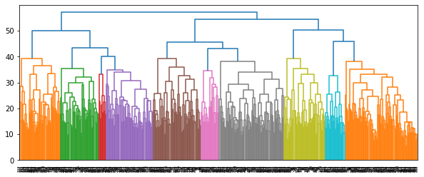
The 3rd column of the extended linkage matrix is the distance between the two clusters to be merged in each row. The 3rd last merge has distance 50.3388, indicating that if the dendrogram is cut at a threshold slightly above 50.3388, there will be 3 clusters.

The format of the extended linkage matrix is detailed in the quick start guide and the Scipy documentation.

from pandas import DataFrame

DataFrame(Z[-3:, :], columns=['x', 'y', 'distance', 'n_pts', 'prototype'])

	x	y	distance	n_pts	prototype
0	1072.0	1078.0	50.338852	182.0	135.0
1	1077.0	1080.0	54.488531	360.0	137.0
2	1079.0	1081.0	57.122675	542.0	22.0

The cluster and prototypes is computed by pyminimax.fcluster_prototype and put together with the target column. The result is sorted by target for better visualization. As expected, most of the images of 1 are in the same cluster (cluster #3), and most of the images of 7 are in a different cluster (cluster #1).

from pyminimax import fcluster_prototype

clust, proto = fcluster_prototype(Z, t=52, criterion='distance').T

res = digits147.assign(clust=clust, proto=proto)
res = res[['target', 'clust', 'proto']].sort_values(by='target')
res

	target	clust	proto
0	1	3	135
154	1	3	135
157	1	3	135
160	1	3	135
379	1	3	135
...	...	...	...
414	7	1	341
126	7	1	341
314	7	1	341
138	7	1	341
136	7	1	341

542 rows × 3 columns

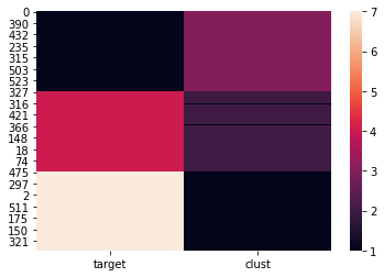
An even better visualization is the below heat map of the target column and the cluster column. It is clear that all images of 1 are in cluster #3, all images of 7 are in cluster #1, and most of images of 4 are in cluster #2. There are only a few images of 4 wrongly put into cluster #1. That is, minimax linkage clustering finds those images closer to 7.

import seaborn as sns

sns.heatmap(res[['target', 'clust']]);

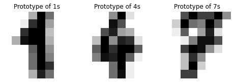
The prototypes are the 135th, 341st, and 464th row of the original DataFrame digits147.

import numpy as np

protos = np.unique(res['proto'])
protos

array([135, 341, 464], dtype=int32)

We print out the images of the prototypes. These are the representative images of 1, 4 and 7.

fig, axs = plt.subplots(nrows=1, ncols=3, figsize=(8, 3))

for ax, proto, label in zip(axs, protos[[0, 2, 1]], [1, 4, 7]):
    ax.set_axis_off()
    image = digits147.drop('target', axis=1).iloc[proto].values.reshape(8, 8)
    ax.imshow(image, cmap=plt.cm.gray_r, interpolation='nearest')
    ax.set_title(f'Prototype of {label}s')

There are 3 images of 4 considered closer to 7. Their indices are 482, 488 and 501, given which we can print out the images for inspection.

res[(res['target']==4) & (res['clust']==1)]

	target	clust	proto
501	4	1	341
488	4	1	341
482	4	1	341

Arguably they are indeed closer to 7’s prototype than 4’s.

fig, axs = plt.subplots(nrows=1, ncols=3, figsize=(8, 3))
plt.suptitle("Images of 4 that are considered closer to 7 by minimax linkage clustering")

for ax, idx in zip(axs, [501, 488, 482]):
    ax.set_axis_off()
    image = digits147.drop('target', axis=1).iloc[idx].values.reshape(8, 8)
    ax.imshow(image, cmap=plt.cm.gray_r, interpolation='nearest')