Quick Start
![]()
![]()
This page is generated by a Jupyter notebook which can be opened and run in Binder or Google Colab by clicking on the above badges. To run it in Google Colab, you need to install PyMinimax in Colab first.
Installation
The recommended way to install PyMinimax is using pip:
[ ]:
pip install pyminimax
Or if you have installed PyMinimax before, please update to the latest version:
[ ]:
pip install --upgrade pyminimax
PyMinimax runs on any platform with Python 3 and SciPy installed.
Usage
The most important function in PyMinimax is pyminimax.minimax, and by default its usage is the same as the hierarchical clustering methods in SciPy, say scipy.cluster.hierarchy.complete. Here we demonstrate with an example from the SciPy documentation. First consider a dataset of \(n=12\) points:
[1]:
X = [[0, 0], [0, 1], [1, 0],
     [0, 4], [0, 3], [1, 4],
     [4, 0], [3, 0], [4, 1],
     [4, 4], [3, 4], [4, 3]]
x x    x x
x        x

x        x
x x    x x
The minimax function takes a flattened distance matrix of the data as an argument, which can be computed by scipy.spatial.distance.pdist. By default, the return value of minimax has the same format as that of scipy.cluster.hierarchy.linkage. This is an \((n-1)\) by 4 matrix keeping the clustering result, called the linkage matrix. A detailed explanation of its format can be found in the SciPy
documentation.
[2]:
from pyminimax import minimax
from scipy.spatial.distance import pdist

Z = minimax(pdist(X))
Z
[2]:
array([[ 0.        ,  1.        ,  1.        ,  2.        ],
       [ 2.        , 12.        ,  1.        ,  3.        ],
       [ 3.        ,  4.        ,  1.        ,  2.        ],
       [ 6.        ,  7.        ,  1.        ,  2.        ],
       [ 5.        , 14.        ,  1.        ,  3.        ],
       [ 8.        , 15.        ,  1.        ,  3.        ],
       [ 9.        , 10.        ,  1.        ,  2.        ],
       [11.        , 18.        ,  1.        ,  3.        ],
       [13.        , 16.        ,  3.16227766,  6.        ],
       [17.        , 19.        ,  3.16227766,  6.        ],
       [20.        , 21.        ,  5.        , 12.        ]])
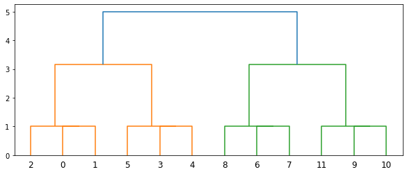
Given the linkage matrix, one can then utilize the methods in SciPy to present the clustering result in a more readable manner. Below are examples applying dendrogram and fcluster.
[3]:
from scipy.cluster.hierarchy import dendrogram
from matplotlib import pyplot as plt

fig = plt.figure(figsize=(10, 4))
dendrogram(Z)
plt.show()
[4]:
from scipy.cluster.hierarchy import fcluster

fcluster(Z, t=1.8, criterion='distance')
[4]:
array([1, 1, 1, 2, 2, 2, 3, 3, 3, 4, 4, 4], dtype=int32)
The above result says that, cutting the dendrogram at 1.8 threshold, the data has 4 clusters, with the first 3 points being in the first cluster, and the following 3 in the second cluster, and so on.
Getting Prototypes
A unique advantage of minimax linkage hierarchical clustering is that in each cluster one prototype is selected from the original data. Thus the resulting clusters are better interpretable. Starting 0.1.2, PyMinimax can also compute those prototypes. Below we demonstrate how this can be done.
To obtain the prototypes, first we need an extended linkage matrix that contains prototypes information. This is an \((n-1)\) by \(5\) matrix, where the first 4 columns are in the same format as the standard linkage matrix and the 5th column keeps the indices of the prototypes of each merged cluster. The extended linkage matrix can be computed by pyminimax.minimax with return_prototype=True.
[5]:
Z_ext = minimax(pdist(X), return_prototype=True)
Z_ext
[5]:
array([[ 0.        ,  1.        ,  1.        ,  2.        ,  0.        ],
       [ 2.        , 12.        ,  1.        ,  3.        ,  0.        ],
       [ 3.        ,  4.        ,  1.        ,  2.        ,  3.        ],
       [ 6.        ,  7.        ,  1.        ,  2.        ,  6.        ],
       [ 5.        , 14.        ,  1.        ,  3.        ,  3.        ],
       [ 8.        , 15.        ,  1.        ,  3.        ,  6.        ],
       [ 9.        , 10.        ,  1.        ,  2.        ,  9.        ],
       [11.        , 18.        ,  1.        ,  3.        ,  9.        ],
       [13.        , 16.        ,  3.16227766,  6.        ,  1.        ],
       [17.        , 19.        ,  3.16227766,  6.        ,  8.        ],
       [20.        , 21.        ,  5.        , 12.        ,  1.        ]])
The 5-column extended linkage matrix is no longer SciPy-compatible. Any SciPy function that takes a linkage matrix will only work if we slice the extended linkage matrix to drop the 5th column, hence the Z_ext[:, :4] below.
[6]:
fig = plt.figure(figsize=(10, 4))
dendrogram(Z_ext[:, :4])
plt.show()

In PyMinimax, the prototypes are computed by pyminimax.fcluster_prototype. Its usage is exactly the same as scipy.cluster.hierarchy.fcluster, except
it takes the 5-column extended linkage matrix instead of a standard 4-column one, and
it returns information regarding clusters and prototypes.
[7]:
from pyminimax import fcluster_prototype

fcluster_prototype(Z_ext, t=1.8, criterion='distance')
[7]:
array([[1, 0],
       [1, 0],
       [1, 0],
       [2, 3],
       [2, 3],
       [2, 3],
       [3, 6],
       [3, 6],
       [3, 6],
       [4, 9],
       [4, 9],
       [4, 9]], dtype=int32)
The above result says that, cutting the dendrogram at 1.8 threshold, the data has 4 clusters. The first 3 points are in the first cluster and the prototype of this cluster is the 0th data point, the following 3 points are in the second cluster and the prototype of this cluster is the 3rd data point, and so on.